D3 Visualization of the Median Market Value of Two Bedroom Homes within some LA Neighborhoods

I have picked the median market values of two bedroom homes within seven LA counties to visualize them over time and compare them with each other.

The counties that I have chosen are:

  1. Beverly Hills (of course, why not),
  2. Santa Monica (this area is really fancy too),
  3. Downtown Los Angeles
  4. West Los Angeles
  5. Culver City
  6. Brentwood
  7. Westwood

As you can see from the above chart, there is basically the same pattern of the median market value of two bedroom homes within each chosen LA neighborhood, and I really like the prices back in 2000.

Continue reading ‘D3 Visualization of the Median Market Value of Two Bedroom Homes within some LA Neighborhoods’ »

Turn Google Analytics Numbers into Actions with Tableau

Recently I have been playing a lot with Tableau, and I decided to extract data from my Google Analytics Account in regard to one of my blogs and visualize the extracted data. Today I want to share my findings. Every visualization gives us some insights into the data. Data connection with Google Analytics opens pretty quick. You can select up 7 dimensions and 10 measures to work with.

The blog is about traveling, and it’s in Russian. Its main audience is in Russia, Eastern Europe, and United States. Below you can see number of sessions, pageviews, and new users by country and year quarter as well as a map.

1_Sessions

1

2_Map Sessions

2

The bubble and waterfall charts below is basically showing the same information, but I like how they look 🙂  The waterfall chart shows the number of organic searches by country. We can see that although the U.S. is the third country by number of pageviews, it’s the second country by the number of organic searches. And Belarus where I am from is the second by number of pageviews, but the forth by the number of organic searches. I guess my friends and family from Belarus influenced this result.

3_Bubble Chart GA

3

4_Waterfall Chart Organic Searches

4

Continue reading ‘Turn Google Analytics Numbers into Actions with Tableau’ »

How to extract Google Analytics data in R and Excel

You will need RGoogleAnalytics package to extract Google Analytics data in R. The package was developed by Michael Pearmain, and it provides functions for accessing and retrieving data from the Google Analytics API. This article is based on the package’s supporting documentation. To download the documentation use this link: RGoogleAnalytics documentation.

First, install the package RgoogleAnalytics. It requires the packages “lubridate” and “httr” to be installed as well.

install.packages("RGoogleAnalytics")
install.packages("lubridate")
install.packages("httr")

library(RGoogleAnalytics)
library(lubridate)
library(httr)

If you have problems with downloading the packages, check your R version. RGoogleAnalytics requires R version 3.0.2 or newer.

Then, you will use the Auth function to authorize the RGoogleAnalytics package to your Google Analytics Account using Oauth2.0.
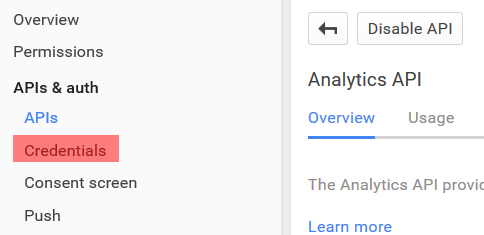
The function Auth expects a Client ID and Client Secret. To get these, you will have to register an application with the Google Analytics API:
1. Go to the Google Developers Console
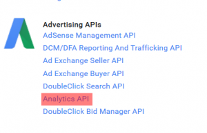
2. Create a New Project and enable the Google Analytics API
3. On the Credentials screen, create a new Client ID for Application Type “Installed Application”
4. Copy the Client ID and Client Secret to your R Script

1_AnalyticsAPI

Enable Google Analytics API

2_Credentials

Create a new Client ID


Now you can authorize the RGoogleAnalytics package to your Google Analytics Account.

client.id <- "your_client_ID_here"
client.secret <- "your_client_secret_here"
token <- Auth(client.id, client.secret)

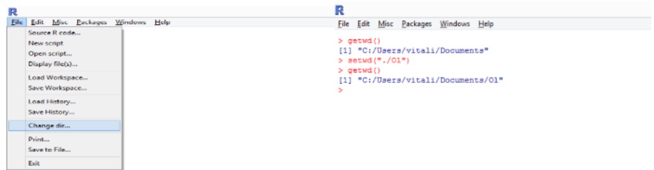
Save the token into the file

save(token,file="./token")

Continue reading ‘How to extract Google Analytics data in R and Excel’ »

Magento MySQL – The most popular sold product per day

I would like to create “The most popular sold product per day” report  for the last 30 days. The header of the report should look like the picture below. We need the Date, Product SKU number, Product name, Product Brand and Quantity Sold. The most popular product is the product sold the maximum number of times on that day.
Header


SELECT CreatedAt, sku AS SKU, name AS Description,
 eaov.value AS Brand, MAX( qty_total ) AS Qty
FROM (

SELECT DATE( created_at ) AS CreatedAt, sku,
 SUM( qty_ordered ) AS qty_total, name, product_id
FROM `sales_flat_order_item` AS sfoi
WHERE sfoi.created_at > DATE_SUB( CURDATE( ) , INTERVAL 360 DAY )
GROUP BY sku, CreatedAt
ORDER BY qty_total DESC
) AS item_count
/* get brand name*/
LEFT JOIN `catalog_product_entity_int` AS cpei ON cpei.attribute_id =81
 AND cpei.entity_id = item_count.product_id
LEFT JOIN `eav_attribute_option_value` AS eaov ON eaov.option_id = cpei.value
GROUP BY CreatedAt

Disadvantage: if two product are equally popular, only one of them is chosen for the report.

Place the results of a MySQL query into a CSV file

The results of a MySQL query can be placed into a CSV file using the following query:

INTO OUTFILE 'file_path'
FIELDS TERMINATED BY ','
ENCLOSED BY '"'
LINES TERMINATED BY '\n';

To include header write another query before the “main” query. It returns the header, and the “main” query returns the data. Union joins them together:

SELECT 'COLUMN1_NAME', 'COLUMN2_NAME'
UNION 
… Your MySQL query here;

View on Github

Magento MySQL – CURDATE() vs NOW()

The CURDATE() function returns the current date.
The NOW() function returns the current system date and time.
If you want to get a sales report for the last X days, make sure to think first what kind of output you want to get.
For me, if I run the same sales report for the last X days in the morning and in the evening of the same day, I want to get the same report without regard the current time, so I will use the CURDATE() function.
In case if we use the NOW() function, and two people want to generate the same report and then do something with it, each of them will get a slightly different version of the report since it’s nearly impossible to run the SQL query at the same time by two different people. It will create discrepancies.
Example: Orders report for the last X days

SELECT SFO.increment_id AS OrderId, SFO.base_subtotal AS BasketAmount, 
	SFO.base_shipping_amount AS Shipping, 	
    SFO.base_discount_amount AS Discount, 
	SFO.base_tax_amount AS Tax, 
    IFNULL( SFO.base_total_paid, 0 ) AS CustomerPaid
FROM  `sales_flat_order` AS SFO
WHERE 
	SFO.created_at > DATE_SUB( CURDATE( ) , INTERVAL X DAY ) 
ORDER BY SFO.created_at DESC  

View on Github

Magento SQL – Five most popular products in general

SELECT sfoi.sku AS SKU, sum(qty_ordered) AS Qty , name AS Description
FROM  `sales_flat_order_item` AS sfoi
JOIN  `catalog_product_entity` AS cpe ON cpe.entity_id = sfoi.product_id
GROUP BY product_id
ORDER BY sum(qty_ordered) DESC
LIMIT 5

However this query does not address the situation when we have more than five most popular product with the same number of units sold. If we have two products that were sold equal number of times, ‘Top Product Number Five’ and ‘Top Product Number 6’, MySQL will return either the ‘Top Product Number Five’ or the ‘Top Product Number 6’ randomly for the fifth most popular product each time we run the query.
View on Github

Magento MySQL – Calculate average number of orders per day and per month

What is the average number of orders per day?

SELECT AVG( orders_num )
FROM (
SELECT created_at, COUNT( DISTINCT order_id ) orders_num
FROM `sales_flat_order_item`
GROUP BY CAST( created_at AS DATE )
)orders_per_day

What is the average number of orders per month?

SELECT AVG( orders_num ) 
FROM (
SELECT created_at, COUNT( DISTINCT order_id ) orders_num
FROM  `sales_flat_order_item` 
GROUP BY MONTH( created_at )
)orders_per_month

View on Github

Multi-family Building Acquisition Financial Modeling

The general idea of the model is to determine the financial feasibility of a Multi-family Building Acquisition Project.

The building is located in Los Feliz, Los Angeles. It has five units, four two-bedroom and a one-bedroom unit. Follow the link to see more information: Multi-family building in Los Feliz.

Multi-family buildings are usually purchased with the intent to lease and produce income to the owner as well as with the expectation of price appreciation of the property.

Assumptions of the model are:

  • Monthly rent
  • Expenses
  • Capitalization Rate
  • Holding Period and
  • Vacancy and Non-payment Rate

Special attention should be given to these assumptions. For example, with the small changes in the Capitalization Rate or Vacancy Rate, the overall profitability of the project may change substantially.
Continue reading ‘Multi-family Building Acquisition Financial Modeling’ »

Getting data from the Web with R and some basic functionality

We will load a dataset into R and do some manipulations in order to show some basic functionality.

The dataset can be downloaded here http://www.bls.gov/oes/current/oes_ca.htm#15-0000. This dataset is a subset of the May 2014 State Occupational Employment and Wage Estimates Report in California by Computer and Mathematical Occupations. The original dataset can be found here http://www.bls.gov/oes/current/oes_ca.htm#(8).

salaries_pic1

  1. The dataset has to be downloaded in your working directory. Getwd() funcion returns an absolute filepath representing the current working directory of the R process. To change your working directory in R you need to use setwd(dir) function or go to the File menu in the R Cosole and choose “Change dir”.
  2. Create a directory for the data
if(!file.exists("salaries")) {
   dir.create("salaries")
}
  1. Download the file
fileUrl < - "your link here"
download.file(fileUrl,destfile = "./salaries/computer.xls")
  1. Next step is to install the xlsx R package if you have not done so previously. To install xlsx, use install.packages(“xlsx”), to ensure if you have it or no, enter find.package(“xlsx”) in the console. After xlsx is done installing, load it using library(xlsx).
  2. Read the file
salariesData <-read.xlsx("./salaries/computer.xls",
                         sheetIndex=1,
                         header=TRUE)
head(salariesData)

salaries_pic2
Continue reading ‘Getting data from the Web with R and some basic functionality’ »

How to subset data in R

How to subset a certain column

data.frame$variable.name

or

data.frame[ , # of the column]

or

data.frame[ , "variable.name"]

All three options above are the same, we are choosing a certain column. For example, if we have a data frame survey which consists of 1,000 observations, and each observation is described by 3 variables: gender, age, and marital status, by using survey$age we can subset the column named “age” for all 1,000 observations.

Continue reading ‘How to subset data in R’ »